

Basics of the Smoothed Particle Hydrodynamics (SPH) Method
This two-part blog series will familiarize you with the basics of the Smoothed Particle Hydrodynamics (SPH) method, discuss some of its advantages and disadvantages over the more traditional Finite Volume (FV) numerical methods, and say a few words of
the SPH implementation in nanoFluidX.
In order to avoid cumbersome reference insertions, we would like to point the interested reader to some of the literature which was used in creating this introductory text and which can provide a far more
detailed insight into the method. Some good places to start are two papers written by Price [1] [2], where he derives the SPH equations and discusses some curiosities of the method in a very accessible way. Adami’s dissertation [3] is a
good reference for those that are interested in particular SPH implementation of nFX. For those wanting to know more about the turbulent behavior, we recommend reading another paper by Adami [4]. Other good reads include the seminal works of Lucy
[5] and Gingold and Monaghan [6], the founders of the method.
Basic Concept of Smoothed Particle Hydrodynamics
The idea of SPH is a very simple one, and it starts by asking how we can reconstruct a continuous field from a cloud of discrete particles which are the property carriers. The problem is 3-dimensional and the solution to our problem should be independent of time. Upon closer thinking, one can pose this as a 3D interpolation problem – interpolating scattered data such that we can reconstruct a continuous field at any point in space and time.
Let us now try to tackle the same problem in 2D, which will help us illustrate the point for 3D as well. Figure 1 below shows how SPH works in 2D – we represent each particle not as a Kroenecker delta function (sharp signal function), but we introduce a Gaussian-like function to smoothen the particle representation, thus the name “smoothed“ particle hydrodynamics. The length across which we smoothen each particle is called the smoothing length and the Gaussian-like function is called a kernel function. By stacking these smoothed particles together, you see that in the bulk we reconstruct a constant and continuous function, which is precisely what we set out to do in the first place.
Figure 1: Reconstruction of a continuous function in 2D using different Gaussian-like curves (kernel functions).
We will stick to the 2D representation for a bit longer to point out a few things. First, note that changing the kernel function and the smoothing length can have a profound impact on the resulting value of the reconstructed field. Second, one can quickly conclude that the particle distribution along the axis can have big influence on the outcome of the reconstruction. Third, it is not perhaps obvious from the figure, but the particle distribution has an impact on the property gradient too. In summary, in SPH the particle distribution and the kernel function properties are critical for obtaining an accurate field reconstruction.
In 3D the principle does not change. The only thing that really changes is the ability to conveniently represent a 3D SPH particle on a 2D screen/paper.
Now, we will assign actual properties to each of the particles, such as mass, pressure, velocity, density and thus volume. Let us also make the kernel function such that the total integral of the volume defined by the smoothing length radius is equal
to 1. Another condition we will force the kernel function to satisfy is that several other, neighboring, particles are encircled by the radius of the smoothing length. This would mean that we can reconstruct any property, e.g. pressure, by
taking the volumetric integral of the kernel function multiplied by the local value of the pressure. In equation form this would look like: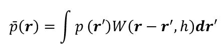
where p̄ is the reconstructed pressure, r is the position vector, r1 is the position vector of the point within the smoothing length radius, h is the smoothing length and W is the kernel function. When you discretize this in terms of SPH, you get:
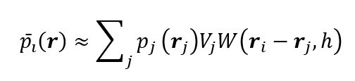
Where the index stands for the so-called owner particle (particle where we are reconstructing the field) and the index for the so-called neighbor particle. Note that in the discretized version of the equation we include , which is volume of the neighbor particle, in order to account for the fact that it is an approximation of the volumetric integral. This also implies that the unit of the kernel summation is 1/volume. We can use the above described principle to reconstruct any of the properties, iwherncluding velocity, density, temperature etc. at any given point in space and time.
Bottom line – SPH is a method based on 3D interpolation of variables through use of specific kernel functions. We weigh the influence of the neighboring particles on the owner particle and repeat this across the domain, where each particle becomes an owner particle at some point.
How Do Things Move in Smoothed Particle Hydrodynamics?
Above we have described the underlying principle of SPH, but we said nothing about how gradients are formed or what causes things to move. This is actually rather easy since it can be shown that the gradient of any variable can be expressed by performing
the same summation as for the normal reconstruction, with the difference of including instead of . Note that the kernel function is almost always a polynomial function and taking its derivative can be done analytically, which is very convenient
for coding. Here’s how the pressure gradient looks in discrete form:

Rather easy, isn’t it? But where does the pressure difference initially come from? The answer to this question is pretty straightforward and it has to do with the particle distribution, which is why we spent some time emphasizing its importance.
Namely, most common approach to SPH is the weakly-compressible method. This approximation usually encompasses simulating incompressible fluids, but artificially allowing them to compress by about 1% of their original density value. This effectively decreases the speed of sound in the simulated fluid and relaxes the numerical conditions for the time step size.
Now, we already said that the particle distribution is critical to the field reconstruction. Let us imagine we are reconstructing the density field and start from a uniform particle distribution in 3D (uniform density). If we now displace a portion of the particles very slightly one way, the total value of the local integral will also increase. This will in turn locally produce a higher density region and, assuming a constant volume of the domain, a rarefaction zone on the opposite side. We can then couple the density change to the pressure change through a quasi-incompressible equation of state, also known as the Tait equation in SPH:

where is the numerical starting pressure, is the so-called background pressure, is the stiffness exponent, is the current density of the owner particle based on the summation and is the default value of the fluid density.
For more detailed explanation of the and please refer to the literature specified at the start.
So, the process is such that we actually reconstruct the density field first and then, based on the density fluctuation, we compute the
pressure for each particle using the Tait equation above. We then take the gradient of the pressure field, as described above and wind up with a driving force for the flow.
Finally, skipping ahead a bit, we show the actual form of the particle
acceleration, which is simply a Navier-Stokes equation we solve for explicitly
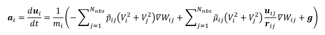
which is, when written in this form, simply Newton’s 2nd Law

While the above form of the acceleration shows some differences on the right-hand side with respect to the original equations we have shown earlier, note that these are just minor corrections introduced to ensure symmetry of the forces and enhance accuracy of the derivatives. Please see the references for additional details.
Of course, this acceleration is then integrated in time to obtain velocity and further shift the particle positions, in turn changing the particle (density) distribution and providing a scene for a new loop of pressure updates and driving force for the flow.
Check back in next Wednesday for part two of this series which examines the advantages and disadvantages of SPH compared to finite volume numerical methods. To learn more about nanoFluidX, please contact your nearest Altair office or visit: altairhyperworks.com/nanofluidx
This guest contribution is written by Milos Stanic, Ph.D., Product Manager – nanoFluidX (nFX) at FluiDyna GmbH. nanoFluidX is a cutting-edge industrial SPH code, developed by FluiDyna GmbH, Germany. Altair is an exclusive World-wide distributor of the nFX software and you can find more information here.
References
| [1] | D. J. Price, "Smoothed particle hydrodynamics and magnetohydrodynamics," Journal of Computational Physics , vol. 231, pp. 759-794, 2012. |
| [2] | D. J. Price, "Smoothed Particle Hydrodynamics: Things I wish my mother taught me," 11 2011. |
| [3] | S. Adami, Modeling and Simulation of Multiphase Phenomena with Smoothed Particle Hydrodynamics, Lehrstuhl für Aerodynamik und Strömungsmechanik, Technische Universität München, 2014. |
| [4] | S. Adami, X. Hu and N. Adams, "Simulating three-dimensional turbulence with SPH," in Proceedings of the Summer Program 2012, Stanford Univeristy, Paolo Alto, 2012. |
| [5] | L. Lucy, "A numerical approach to the testing of the fission hypothesis," Astronomical Journal, vol. 82, pp. 1013-1024, #dec# 1977. |
| [6] | R. Gingold and J. Monaghan, "Smoothed particle hydrodynamics - Theory and application to non-spherical stars,"Monthly Notices of the Royal Astronomical Society, vol. 181, pp. 375-389, #nov# 1977. |
| [7] | A. Kajzer, J. Pozorski and K. Szewc, "Large-eddy simulations of 3D Taylor-Green vortex: comparison of Smoothed Particle Hydrodynamics, Lattice Boltzmann and Finite Volume methods," Journal of Physics: Conference Series, vol. 530, p. 012019, 2014. |

